Twitter Mood Predicts Stock Market Movement

Download: mood_dataset.zip

In this post, I try to predict the daily up and down movement of stock prices using twitter mood data and machine learning algorithms. Some time ago, I read a paper called “Twitter mood predicts the stock market.” They claimed to be able to predict stock price movement with an accuracy of over 86%. They used 9,853,498 tweets posted by 2.7 million English speaking users in 2008 and showed that general twitter mood could be used to predict the DJIA. 

My initial intention was to reproduce their results. However, their method would have required that I have access to large scale historical twitter data which is not free and probably not cheap. Instead, I found two companies that publish daily mood sentiment for individual stocks with historical data going back a couple of months. You can download here the anonymized dataset I used for IBM and AGN. I have anonymized the dataset for two reasons; I don’t know if it is legal to share this data and secondly, I might decide to use this method for my own financial gain – the results are impressive! 

For the first company that publishes mood data, I  combine the mood data for the previous 2, 5, and 8 days to predict whether a stock price goes up, down or stays flat. The accuracy is around 75% for AGN and 80% for IBM using 8 days of mood data. For the second company that publishes mood data the results where very impressive; around 90%-100% accuracy using just the previous day's mood data for all the stocks I tested. Below are the results summarized in a confusion matrix.

I used a decision tree and 5x cross-validation for all tests.

Company (1) $AGN Confusion Matrix with 2 days worth of mood data   down     flat     up   down 55.1 % 0.0 % 44.9 % 205 flat 33.3 % 0.0 % 66.7 % 3 up 35.9 % 0.0 % 64.1 % 234 198 0 244 442 Note: columns represent predictions, row represent true classes $AGN Confusion Matrix with 5 days worth of mood data   down     flat     up   down 71.7 %  0.0 %  28.3 %  205 flat 66.7 %  0.0 %  33.3 %  3 up 23.7 %  0.0 %  76.3 %  232 204 0 236 440 Note: columns represent predictions, row represent true classes $AGN Confusion Matrix with 8 days worth of mood data   down     flat     up   down 74.9 %  0.0 %  25.1 %  203 flat 0.0 %  0.0 %  100.0 %  3 up 23.5 %  0.4 %  76.1 %  230 206 1 229 436 Note: columns represent predictions, row represent true classes $IBM Confusion Matrix with 8 days worth of mood data   down     flat     up   down 82.8 %  0.0 %  17.2 %  215 flat N/A %  N/A %  N/A %  0 up 20.1 %  0.0 %  79.9 %  249 228 0 236 464 Note: columns represent predictions, row represent true classes Company (2) $AGN Confusion Matrix with 1 day worth of mood data   down     flat     up   down 100.0%  0.0 %  44.9 %  460 flat 0.0 %  100.0 %  0.0 %  46 up 0.0 %  0.0 %  100.0 %  436 460 46 436 942 Note: columns represent predictions, row represent true classes

Read More

Experiments with Real-time Linux

After installing real-time linux on both my Ubuntu laptops, my goal was to get a feel for how well latency peaks are eliminated compared to the standard Linux kernel. I was specificaly interested in network port latencies. Before looking at the network specific latenicies, I experimented with the internal worst-case interrupt latency of the kernel. The worst case latency for each hardware device will differ. The latencies of interrupts for devices connected directly to the CPU (e.g. local APIC) will be lower than the latencies of interrupts for devices connected to the CPU through a PCI bus. The interrupt latency for the APIC timer can be measured using "cyclictest". This should provide the lower-bound for interrupt latencies. Most likely, all other interrupts generated by other devices including the network card will exceed this value. The goal of running an RT kernel is to make the response time more consistent, even under load. I used hackbench to load the CPUs. You can see the effect on each processor by running htop:

hackbench -l 10000

htop

  1  [|||||||||||||||||||||||||||||||||||||||||||||||||||||||||||||||||||||||||||||||||||||||||||98.1%]    
  2  [|||||||||||||||||||||||||||||||||||||||||||||||||||||||||||||||||||||||||||||||||||||||||||98.7%]    
  3  [|||||||||||||||||||||||||||||||||||||||||||||||||||||||||||||||||||||||||||||||||||||||||||98.7%]    
  4  [||||||||||||||||||||||||||||||||||||||||||||||||||||||||||||||||||||||||||||||||||||||||||100.0%]
  5  [|||||||||||||||||||||||||||||||||||||||||||||||||||||||||||||||||||||||||||||||||||||||||||97.5%]
  6  [|||||||||||||||||||||||||||||||||||||||||||||||||||||||||||||||||||||||||||||||||||||||||||97.5%]
  7  [|||||||||||||||||||||||||||||||||||||||||||||||||||||||||||||||||||||||||||||||||||||||||||99.4%]
  8  [||||||||||||||||||||||||||||||||||||||||||||||||||||||||||||||||||||||||||||||||||||||||||100.0%]
  Mem[|||||||||||||||||||||||||||||||||||||||||                                            1036/7905MB]
  Swp[                                                                                       0/16210MB]

  PID USER     PRI  NI  VIRT   RES   SHR S CPU% MEM%   TIME+  Command
 2843 dimitri   20   0  545M 75140 22716 S  4.0  0.9  1:21.71 /usr/bin/python /usr/bin/deluge-gtk
20586 dimitri   20   0 29500  2272  1344 R  3.0  0.0  0:00.91 htop
20896 root      20   0  6332   116     0 S  3.0  0.0  0:00.19 hackbench -l 10000
20884 root      20   0  6332   116     0 S  3.0  0.0  0:00.19 hackbench -l 10000
20969 root      20   0  6332   116     0 S  3.0  0.0  0:00.17 hackbench -l 10000
20885 root      20   0  6332   116     0 S  2.0  0.0  0:00.19 hackbench -l 10000
20895 root      20   0  6332   116     0 R  2.0  0.0  0:00.19 hackbench -l 10000
20883 root      20   0  6332   116     0 S  2.0  0.0  0:00.19 hackbench -l 10000
20891 root      20   0  6332   116     0 S  2.0  0.0  0:00.19 hackbench -l 10000
20682 root      20   0  6332   112     0 S  2.0  0.0  0:00.21 hackbench -l 10000
20715 root      20   0  6332   112     0 D  2.0  0.0  0:00.19 hackbench -l 10000
20887 root      20   0  6332   116     0 S  2.0  0.0  0:00.19 hackbench -l 10000
20911 root      20   0  6332   116     0 D  2.0  0.0  0:00.18 hackbench -l 10000
20880 root      20   0  6332   116     0 D  2.0  0.0  0:00.18 hackbench -l 10000
20881 root      20   0  6332   116     0 S  2.0  0.0  0:00.19 hackbench -l 10000
20882 root      20   0  6332   116     0 S  2.0  0.0  0:00.18 hackbench -l 10000
20888 root      20   0  6332   116     0 R  2.0  0.0  0:00.19 hackbench -l 10000
20889 root      20   0  6332   116     0 R  2.0  0.0  0:00.19 hackbench -l 10000
20890 root      20   0  6332   116     0 S  2.0  0.0  0:00.19 hackbench -l 10000
20892 root      20   0  6332   116     0 S  2.0  0.0  0:00.19 hackbench -l 10000
20894 root      20   0  6332   116     0 S  2.0  0.0  0:00.18 hackbench -l 10000
20897 root      20   0  6332   116     0 S  2.0  0.0  0:00.19 hackbench -l 10000
20898 root      20   0  6332   116     0 S  2.0  0.0  0:00.19 hackbench -l 10000
20912 root      20   0  6332   116     0 R  2.0  0.0  0:00.18 hackbench -l 10000

Hackbench ran all eight CPUs at near 100% and also caused lots of rescheduling interrupts. The scheduler tries to spread processor activity across as many cores as possible. When the scheduler decides to offload work from one core to another core, a rescheduling interrupt occurs. I also attempted to increase other device intrupts by running the bittorrent deluge client and rtsp/rtp internet radio. This generated both sound and wifi (ath9k) interrupts. Below, you can see a snapshot of the interrupt count for each device. The wifi (ath9k) is IRQ 17 and eth0 is on IRQ 56.

watch -n 1 cat /proc/interrupts

           CPU0       CPU1       CPU2       CPU3       CPU4       CPU5       CPU6       CPU7    
  0:        144          0          0          0          0         0         0          0   IO-APIC-edge      timer
  1:         11           0          0          0          0          0         0          0   IO-APIC-edge      i8042
  8:          1            0          0          0          0          0          0          0   IO-APIC-edge      rtc0
  9:        399          0          0          0          0          0         0         0   IO-APIC-fasteoi   acpi
 12:        181         0          0          0          0          0         0         0   IO-APIC-edge      i8042
 16:        114         0        221        0          0          0         0         0   IO-APIC-fasteoi   ehci_hcd:usb1, mei
 17:     238921      0          0          0          0          0         0         0   IO-APIC-fasteoi   ath9k
 23:        113         0      10894      0          0          0         0         0   IO-APIC-fasteoi   ehci_hcd:usb2
 40:          0           0          0            0          0          0         0         0   PCI-MSI-edge      PCIe PME
 41:          0          0          0          0          0          0          0          0   PCI-MSI-edge      PCIe PME
 42:          0          0          0          0          0          0          0          0   PCI-MSI-edge      PCIe PME
 43:          0          0          0          0          0          0          0          0   PCI-MSI-edge      PCIe PME
 44:          0          0          0          0          0          0          0          0   PCI-MSI-edge      PCIe PME
 45:          0          0          0          0          0          0          0          0   PCI-MSI-edge      xhci_hcd
 46:          0          0          0          0          0          0          0          0   PCI-MSI-edge      xhci_hcd
 47:          0          0          0          0          0          0          0          0   PCI-MSI-edge      xhci_hcd
 48:          0          0          0          0          0          0          0          0   PCI-MSI-edge      xhci_hcd
 49:          0          0          0          0          0          0          0          0   PCI-MSI-edge      xhci_hcd
 50:          0          0          0          0          0          0          0          0   PCI-MSI-edge      xhci_hcd
 51:          0          0          0          0          0          0          0          0   PCI-MSI-edge      xhci_hcd
 52:          0          0          0          0          0          0          0          0   PCI-MSI-edge      xhci_hcd
 53:      32389     0          0          0          0          0          0          0   PCI-MSI-edge      ahci
 54:     195410    0          0          0          0          0          0          0   PCI-MSI-edge      i915
 55:        273        6          0          0          0          0          0          0   PCI-MSI-edge      hda_intel
 56:          2          0          0           0          0          0          0          0   PCI-MSI-edge      eth0
NMI:        0         0          0           0          0          0          0          0   Non-maskable interrupts
LOC:    2592013  3074746  2470454  2448349  2525416  2454510  2440296  2424395 Local timer inter
SPU:         0          0          0          0          0          0          0          0   Spurious interrupts
PMI:         0          0          0          0          0          0          0          0   Performance monitoring interrupts
IWI:          0          0          0          0          0          0          0          0   IRQ work interrupts
RES:   357199   449954   390871   399211 536214   606334  493824   554138   Rescheduling interrupts
CAL:       300     467      500     505      480      484   477 476      Function call interrupts
TLB:       2876    647        582   632     1079    663    432   485   TLB shootdowns
TRM:         0          0          0          0          0          0          0          0   Thermal event interrupts
THR:          0          0          0          0          0          0          0          0   Threshold APIC interrupts
MCE:         0          0          0          0          0          0          0          0   Machine check exceptions




After loading the system, I ran cycletest at a very high real-time priority of 99:

On the Preempt-RT linux kernel:

sudo cyclictest -a 0 -t -n -p99
T: 0 ( 3005) P:99 I:1000 C: 140173 Min:      1 Act:    2 Avg:    9 Max:     173
T: 1 ( 3006) P:98 I:1500 C:  93449 Min:      1 Act:    4 Avg:   16 Max:     172
T: 2 ( 3007) P:97 I:2000 C:  70087 Min:      1 Act:    4 Avg:   17 Max:     182
T: 3 ( 3008) P:96 I:2500 C:  56069 Min:      2 Act:   13 Avg:   17 Max:     166
T: 4 ( 3009) P:95 I:3000 C:  46725 Min:      2 Act:    3 Avg:   17 Max:     174
T: 5 ( 3010) P:94 I:3500 C:  40050 Min:      2 Act:   10 Avg:   15 Max:     163
T: 6 ( 3011) P:93 I:4000 C:  35044 Min:      2 Act:    4 Avg:   20 Max:     169
T: 7 ( 3012) P:92 I:4500 C:  31150 Min:      2 Act:   13 Avg:   22 Max:     164


On a standard Linux kernel:

sudo cyclictest -a 0 -t -n -p99

T: 0 ( 4264) P:99 I:1000 C:  76400 Min:      3 Act:    5 Avg:   10 Max:    6079
T: 1 ( 4265) P:98 I:1500 C:  50934 Min:      2 Act:    6 Avg:   13 Max:   15501
T: 2 ( 4266) P:97 I:2000 C:  38201 Min:      3 Act:    6 Avg:    6 Max:    4685
T: 3 ( 4267) P:96 I:2500 C:  30561 Min:      3 Act:    5 Avg:    6 Max:    1735
T: 4 ( 4268) P:95 I:3000 C:  25467 Min:      3 Act:    5 Avg:    6 Max:    1288
T: 5 ( 4269) P:94 I:3500 C:  21829 Min:      3 Act:    7 Avg:    8 Max:   13301
T: 6 ( 4270) P:93 I:4000 C:  19101 Min:      3 Act:    6 Avg:    6 Max:    2192
T: 7 ( 4271) P:92 I:4500 C:  16978 Min:      4 Act:    5 Avg:    6 Max:      85

The maximum latenency for the standard linux kernel is as high as 15501 microseconds and depends on load. The maximum timer latency irrespective of load is between 150 and 185 microseconds for the Preempt-RT linux kernel. The averagae latency, however, is better on the standard linux kernel. This is to be expected as the main goal of the real-time kernel is determinism and performance may or may not suffer. I then connected my two laptops directly via a cross-over network cable and used a modified version of the zeromq performance tests to measure the round-trip latency of both the real-time and standard kernels. Both the sender and receiver test applications where run at a real-time priority of 85.

Sends 50000 packets (1 byte)  and measures round-trip time:

sudo chrt -f 85 ./local_lat tcp://eth0:5555 1 50000


Receives packets and returns them to sender:

sudo chrt -f 85 ./remote_lat tcp://192.168.2.24:5555 1 50000

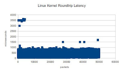
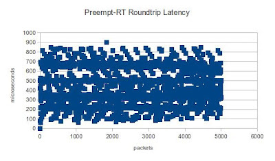
In the diagram below, you can see that the real-time kernel's maximum round-trip packet latencies never exceed 900 microseconds, even under high load. The standard kernel, however, suffered several peaks, some as high as 3500 microseconds.

Preempt-RT Round-trip Latency

Standard Linux Kernel Round-trip Latency

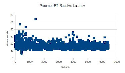
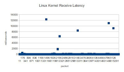
I then used ku-latency application to measure the amount of time it takes the Linux kernel to hand a received network packet off to user space. The real-time kernel never excceds 50 microsecods with an average of around 20 microseconds. The standard kernel, on the other hand, suffered some extreme peaks.

Preempt-RT Receive Latency

Standard Linux Receive Latency

For these experiments, I did not take into account CPU affinity. Different results could be achieved with CPU shielding -- something I might leave for another blog post.

References:

• Myths and Realities of Real-Time Linux Software Systems
• Red Hat Enterprise MRG 1.3 Realtime Tuning Guide
• Best practices for tuning system latency
• https://github.com/koppi/renoise-refcards/wiki/HOWTO-fine-tune-realtime-audio-settings-on-Ubuntu-11.10
• http://sickbits.networklabs.org/configuring-a-network-monitoring-system-sensor-w-pf_ring-on-ubuntu-server-11-04-part-1-interface-configuration/
• http://vilimpoc.org/research/ku-latency/

Read More

Real-time Linux

I installed the RT Linux kernel on both of my Ubuntu laptops recently and I am happy to report that thus far I have not noticed any negative side-effects. The RT patch seems to be stable -- video, sound, networking etc. continue to work as before. My intention is to experiment with the RT kernel. In what way is the network latency affected ? Is the packet latency from the ethernet port to user space predictable ?

Many software applications benefit from a real time operating system. I used to work on aircraft simulators. In order for the pilot to experience smooth motion, frames would have to be updated every 16 milliseconds (60 FPS). Too many consecutive frames dropped, often produced unacceptable jerky motion. A single frame dropped from time to time had no appreciable effect. This is an example of a soft real-time system. The system met the desired deadlines on average. A soft real-time system does not guarantee maximum response time. On the other hand, hard real-time systems meet the desired deadlines at all times, even under a worst-case system load. 

The Linux kernel can be made into a real-time kernel by applying Ingo Molnar’s PREEMPT RT patch. This patch makes a regular Linux kernel into a fully Preemptible OS - an OS that has the capability to stop/hold a low priority task in favour of a high priority task. 

I copy the instructions I used to build and install the patch below.

To build the RT kernel by hand, first install the required software packages:

sudo apt-get install kernel-package fakeroot build-essential libncurses5-dev

Then fetch the vanilla kernel and RT patch (the version numbers are somewhat old, tweak as necessary):

mkdir -p ~/tmp/linux-rt
cd ~/tmp/linux-rt
wget http://www.kernel.org/pub/linux/kernel/v3.x/linux-3.4.tar.bz2
wget http://www.kernel.org/pub/linux/kernel/projects/rt/3.4/patch-3.4-rt7.patch.bz2
tar xjvf linux-3.4.tar.bz2
cd linux-3.4
patch -p1 < <(bunzip2 -c ../patch-3.4-rt7.patch.bz2)

Then configure the kernel using:

cp /boot/config-$(uname -r) .config && make oldconfig

where you should select "full preemption" (option 5) when prompted, and leave everything else at its default value by pressing enter at every prompt. The config from the -lowlatency kernel might be a better starting point than that of the -generic kernel.

Then build the kernel with: 

sed -rie 's/echo "\+"/#echo "\+"/' scripts/setlocalversion
make-kpkg clean
CONCURRENCY_LEVEL=$(getconf _NPROCESSORS_ONLN) fakeroot make-kpkg --initrd --revision=0 kernel_image kernel_headers

And finally install your new kernel with:

sudo dpkg -i ../linux-{headers,image}-3.4-rt7_0_*.deb

Read More

Clustering Through Decision Tree Construction

Download: https://github.com/dimitrs/CLTree

As is often the case, any idea you may have, no matter how novel you may think it is, has already been thought of by someone else. Some time ago I wanted to modify a decision tree induction algorithm for clustering. I thought that this could be a new method for clustering, but fortunately after an internet search, I came across a paper that described a method to do clustering using decision trees called CLTree. I like to re-use what other people have already done – it saves me a lot of time. Sadly, people writing papers do not always provide the source code. However, the paper did provide a fairly detailed description of the algorithm. In this post, I present an implementation of that algorithm.

Here are some of the benefits of this algorithm as described by the paper:

·         CLTree is able to find clusters in the full dimension space as well as in subspaces.

·         It provides descriptions of the resulting clusters in terms of hyper-rectangle regions.

·         It provides descriptions of the resulting empty (sparse) regions.

·         It deals with outliers effectively.

The basic idea is to assign each instance in the dataset a class Y. A decision tree requires at least two classes to partition a dataset. Assume that the data space is uniformly distributed with “other” instances of class N, called non-existing or virtual instances. By adding the N instances to the original dataset, the problem of partitioning the dataset into dense data regions and sparse empty regions becomes a classification problem. For the details please read the paper.

Below, the algorithm found three clusters for the trivial two dimensional dataset (gen.arff) that you can find with the source code I provide.

Please be aware that this implementation has only been tested on a couple of trivial datasets. One with two dimension and the other with five (provided with the source code). It probably will not scale very well with large datasets.

Read More

Use WEKA in your Python code

Weka is a collection of machine learning algorithms that can either be applied directly to a dataset or called from your own Java code. There is an article called “Use WEKA in your Java code” which as its title suggests explains how to use WEKA from your Java code. This is not a surprising thing to do since Weka is implemented in Java. As the title of this post suggests, I will describe how to use WEKA from your Python code instead.

If you have built an entire software system in Python, you might be reluctant to look at libraries in other languages. After all, there are a huge number of excellent Python libraries, and many good machine-learning libraries written in Python or C and C++ with Python bindings. However, as far as I am concerned, it would be a pity not to make use of Weka just because it is written in Java. It is one of the most well known machine-learning libraries around with an extensive number of implemented algorithms. What’s more, there are very few data stream mining libraries around and MOA, related to Weka and also written in Java is the best I have seen.

I use Jpype (http://jpype.sourceforge.net/) to access Weka class libraries. Once you have it installed, download the latest Weka & Moa versions and copy moa.jar, sizeofag.jar and weak.jar into your working directory. Below you can see the full Python listing of the test application. The code initializes the JVM, imports some Weka packages and classes, reads a data set, splits it into a training set and test set, trains a J48 tree classifier and then tests it. If you are familiar with Weka, this will all be very easy.

In a separate post, I will explore how easy it is to use MOA in the same way.

# Initialize the specified JVM
from jpype import *options = [
"-Xmx4G",
"-Djava.class.path=./moa.jar",
"-Djava.class.path=./weka.jar",
"-Djavaagent:sizeofag.jar",
]
startJVM(getDefaultJVMPath(), *options)

# Import java/weka packages and classes
Trees = JPackage("weka.classifiers.trees")
Filter = JClass("weka.filters.Filter")
Attribute = JPackage("weka.filters.unsupervised.attribute")
Instance = JPackage("weka.filters.unsupervised.instance")
RemovePercentage = JClass("weka.filters.unsupervised.instance.RemovePercentage")
Remove = JClass("weka.filters.unsupervised.attribute.Remove")
Classifier = JClass("weka.classifiers.Classifier")
NaiveBayes = JClass("weka.classifiers.bayes.NaiveBayes")
Evaluation = JClass("weka.classifiers.Evaluation")
FilteredClassifier = JClass("weka.classifiers.meta.FilteredClassifier")
Instances = JClass("weka.core.Instances")
BufferedReader = JClass("java.io.BufferedReader")
FileReader = JClass("java.io.FileReader")
Random = JClass("java.util.Random")


#Reading from an ARFF file
reader = BufferedReader(FileReader("./iris.arff"))
data = Instances(reader)
reader.close()
data.setClassIndex(data.numAttributes() - 1) # setting class attribute

# Standardizes all numeric attributes in the given dataset to have zero mean and unit variance, apart from the class attribute.
standardizeFilter = Attribute.Standardize()
standardizeFilter.setInputFormat(data)
data = Filter.useFilter(data, standardizeFilter)

# Randomly shuffles the order of instances passed through it.
randomizeFilter = Instance.Randomize()
randomizeFilter.setInputFormat(data)
data = Filter.useFilter(data, randomizeFilter)

# Creating train set
removeFilter = RemovePercentage()
removeFilter.setInputFormat(data)
removeFilter.setPercentage(30.0)
removeFilter.setInvertSelection(False)
trainData = Filter.useFilter(data, removeFilter)

# Creating test set
removeFilter.setInputFormat(data)
removeFilter.setPercentage(30.0)
removeFilter.setInvertSelection(True)
testData = Filter.useFilter(data, removeFilter)

# Create classifier
j48 = Trees.J48()
j48.setUnpruned(True) # using an unpruned J48
j48.buildClassifier(trainData)

print "Number Training Data", trainData.numInstances(), data.numInstances()
print "Number Test Data", testData.numInstances()

# Test classifier
for i in range(testData.numInstances()):
    pred = j48.classifyInstance(testData.instance(i))
    print "ID:", testData.instance(i).value(0),
    print "actual:", testData.classAttribute().value(int(testData.instance(i).classValue())),
    print "predicted:", testData.classAttribute().value(int(pred))

shutdownJVM()

Read More

Encode and Decode Video from Memory

Download: https://github.com/dimitrs/video_coding

OpenCV provides a very simple api to connect to a camera and show the images in a window. It is also very simple to encode those images and store them on disk. However, the simple api provides no means by which to encode an image without storing it on disk and even worse, no means to decode an image stored in memory instead of on disk. Assuming I want to capture an image from a camera and send it over a socket to a receiver, one might want to first compress the image before sending it. A simple test I did indicated that an image can be compressed by a factor of 10 using the mpeg-4 codec. This is really important for streaming applications.

On Linux and Windows, OpenCV’s underlying implementation uses the ffmpeg library to encode/decode frames to and from disk. I found the implementation in opencv\modules\highgui\src\cap_ffmpeg_impl.hpp. In this post, I provide a small test project with a modified version of cap_ffmpeg_impl.hpp. This version allows you to encode/decode images to and from a buffer instead of disk. Warning: The code is a proof of concept and not production ready. You can find the project in github.

Below, you can see how to encode/decode video:

Initializing capture from a camera:

CvCapture* capture = cvCaptureFromCAM(CV_CAP_ANY);

Capturing a frame:

cvGrabFrame(capture); // capture a frame
IplImage* img = cvRetrieveFrame(capture); // retrieve the captured frame

Initialize a video encoder:

int fps = 10;
int width = 320;
int height = 320;
CvVideoWriter_FFMPEG writer;
writer.init();
writer.open("x.mpg", CV_FOURCC('D', 'I', 'V', 'X'), fps, width, height, true);

Encoding the previously captured image:

int wStep = img->widthStep;
int w =  img->width;
int h = img->height;
int c = img->nChannels;
writer.writeFrame((const uchar*)img->imageData, wStep, w, h, c, img->origin);

Initialize a video decoder:

CvCapture_FFMPEG cap;
cap.open(width, height);

Decoding the previously encoded image:

uint8_t* buffer = &writer.outbuf[0];
int length = writer.out_size;
cap.grabFrame(buffer, length);
IplImage* img2 = cap.retrieveFrame();

Show image in a window:

if (img2)
{
    cvShowImage("My Window", img2 );
    cvWaitKey();
}

Read More

How-to embed HTML in a ReStructuredText PDF document

Download: rst2pdf_html.tar.gz 

I use rst2pdf to create PDF documents from reStructuredtext and on occasion, I have needed to embed HTML in those documents. Unfortunately, this is not possible with rst2pdf as it does not support html embedding. However, with this version of rst2pdf you can embed html as I have done in the example below. The email addresses are rendered as HTML using the “raw:: html” directive. This will only work with this version of rst2pdf and you will need to have xhtml2pdf installed.

ReStructuredtext for the above example:

.. list-table::
   :widths: 50 50 
   :header-rows: 1

   * - **Name**   
     - **e-mail**   
   * - Pedro
     - .. raw:: html
       
         <p><a href="mailto:pedro@address.es">pedro@mailaddress.es</a></p>
   * - Dimitri
     - .. raw:: html
       
         <p><a href="mailto:dimitr@mail.es">dimitr@mailaddress.es</a></p>

Read More